ЖЭТФ, 2022, том 161, вып. 2, стр. 184-188

DIFFERENTIABLE PROGRAMMING

FOR PARTICLE PHYSICS SIMULATIONS

R. Grinis^***

Moscow Institute of Physics and Technology

141700, Dolgoprudny, Moscow Region, Russia

Received August 24, 2021,

revised version August 24, 2021

Accepted for publication October 6, 2021

DOI: 10.31857/S0044451022020043

tial equations started to gather pace with the work of

Chen et al. [1]. A whole new area tagged now-days

Neural Differential Equations arose in scientific ML.

Abstract. We describe how to apply adjoint sen-

sitivity methods to backward Monte-Carlo schemes

On one hand, using ML we obtain a more flexible

arising from simulations of particles passing through

framework with a wealth of new tools to tackle a variety

matter. Relying on this, we demonstrate deriva-

of inverse problems in mathematical modeling. On the

tive based techniques for solving inverse problems for

other hand, many techniques in the latter such as the

such systems without approximations to underlying

adjoint sensitivity methods give rise to new powerful

transport dynamics. We are implementing those al-

algorithms for AD.

gorithms for various scenarios within a general pur-

pose differentiable programming C++17 library NOA

A few implementations are now available:

(github.com/grinisrit/noa).

— torchdiffeq is the initial python package devel-

oped by [1] providing ODE solvers that not only inte-

1. Overview of the main results. In this pa-

grate with PyTorch DL models, but also use those to

per, we explore the challenges and opportunities that

describe the dynamics;

arise in integrating differentiable programming (DP)

with simulations in particle physics.

— torchsde builds off from torchdiffeq and provides

the same functionality for SDEs, as well as O(1)-me-

In our context, we will broadly refer to DP as a pro-

mory gradient computation algorithms, see [2];

gram for which some of the inputs could be given the

notion of a variable, and the output of that program

— diffeqflux is a Julia package developed by Rack-

could be differentiated with respect to them.

auckas et al. [3] and relies on a rich scientific ML ecosys-

tem treating many different types of equations inclu-

Most common examples include the widely used

ding PDEs.

deep learning (DL) models created over the powerful

automatic differentiation (AD) engines such as Tensor-

Unsurprisingly, one can also find roots of this story

Flow and PyTorch. Since their initial release, those ma-

in computational finance, see for example the work of

chine learning (ML) frameworks grew up into fully-fled-

Giles et al. [4]. An AD algorithm is presented there

ged DP libraries capable of tackling a more diversified

for computing the risk sensitivities for a portfolio of

set of tasks.

options priced through Monte-Carlo simulation. That

set-up is close to our case of interest and therefore rep-

Recently, a very fruitful interaction between DP as

resents a great source of inspiration for us.

we know it in ML and numerical solutions to differen-

In fact, for particle physics simulations a similar

^* E-mail: roland.grinis@grinisrit.com

picture is left almost unexplored so far. The dynamics

^** GrinisRIT ltd., London, UK

are richer than the ones considered before, but we also

184

ЖЭТФ, том 161, вып. 2, 2022

Differentiable programming for particle physics simulations

log likelyhood

–0.01

–0.02

–0.03

–0.04

detector

–1

200

400

600

800

1000

–4

-2

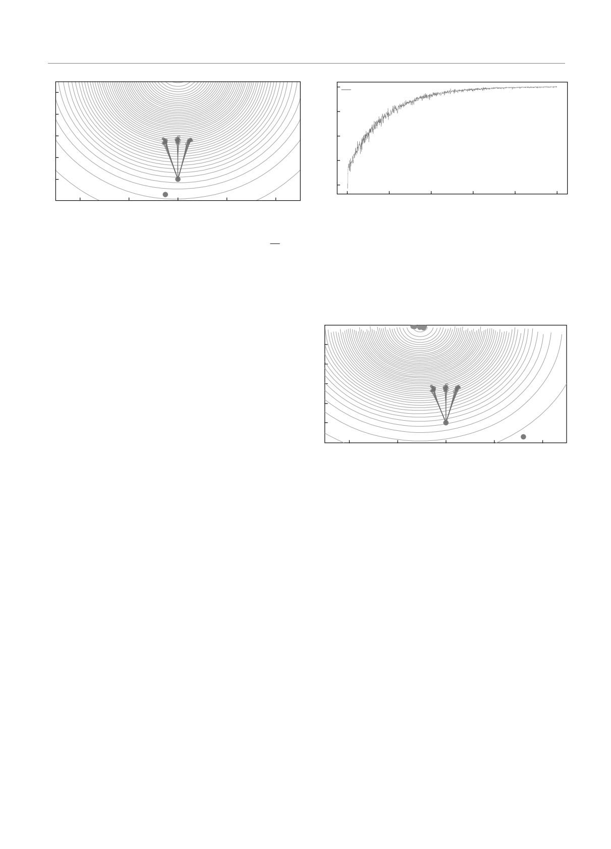
Fig. 2. After implementing BMC over LibTorch’s Autograd li-

Fig. 1. (Color online) This is a toy example. The contours

brary we can use a gradient based optimisation to solve the in-

correspond to level sets of the materials mixture given by a

√

verse problem for ϑμ and ϑσ. Let us set ϑμ = (-1, 5) arbitrar-

Gaussian centered at ϑμ = (0, 5) with scale ϑσ =

10. In

ily. We present SGD convergence over 1000 steps with learning

blue we show the BMC simulated trajectories. For the sake of

rate 0.05, reaching

ϑμ = (-1.0033, 4.9891) and

ϑ2σ = 9.9611

simplicity, we assume the known particle flux is constant equals

in good agreement with true values

to one and is reached after two steps. A naive implementation

of the BMC scheme to compute the flux in this configuration

can be found in the Appendix, routine backward_mc 1.There

is, however, a challenge with the approach consisting in differ-

entiating through the MC simulation with AD. The algorithm is

not scalable in the number of steps for the discretisation of the

transport. This issue can be addressed by adjoint sensitivity

methods. The routine backward_mc_grad 2 in the Appendix

provides an implementation with first order derivative for the

BMC scheme in this example

detector

have more tools at our disposal such as the Backward

–1

–4

Monte-Carlo (BMC) techniques [5, 6]. We make use of

Fig. 3. (Color online) Optimal parameters and Bayesian pos-

the latter to adapt the adjoint sensitivity methods [7] to

terior sampled using NOA [8] implementation of Riemannian

the transport of particles through matter simulations.

HMC with an explicit symplectic integrator

Ultimately, we obtain a novel methodology for

image reconstruction problems when the absorption

mechanism is non-linear. In future, one can demon-

Acknowledgments. I would like to thank the

strate this approach in the specific case of muography.

MIPT-NPM lab and A. Nozik in particular for very

We are releasing our implementations within the open

fruitful discussions that have led to this work. We are

source library NOA [8].

very grateful to GrinisRIT for the support.

The results are shown in Figs. 1-3.

2. Conclusion. In this paper, we have demon-

This work has been initially presented at the

strated how to efficiently integrate automatic diffe-

QUARKS-2020 workshop — serie “Advanced Compu-

rentiation and adjoint sensitivity methods with BMC

ting in Particle Physics”.

schemes arising in the passage of particles through mat-

ter simulations.

The full text of this paper is published in the English

version of JETP.

We believe that this builds a whole new bridge be-

tween scientific machine learning and inverse problems

Appendix. Code examples. We have col-

arising in particle physics. In future, we hope to prove

lected here the two BMC implementations for our

the success of this technique in a variety of image recon-

basic example. You can reproduce all the calcu-

struction problems with non-linear dynamics, starting

lations in this paper from the notebook differen-

with muography.

tiable_programming_pms.ipynb available in NOA [8].

185

ЖЭТФ, вып. 2

R. Grinis

ЖЭТФ, том 161, вып. 2, 2022

For the specific code snippets here the only dependency is LibTorch:

#include

The following routine will be used throughout and provides the rotations by a tensor angles for multiple

scattering:

inline torch :: Tensor rot(const torch :: Tensor &angles)

{

const auto n = angles .numel();

const auto c = torch :: cos(angles );

const auto s = torch :: sin(angles );

return torch :: stack({c, -s , s , c } ). t ( ) . view ({n ,

2});

}

Given the set-up in Fig. 1 example we define:

const auto detector

= torch :: zeros(2);

const auto materialA = 0.9f;

const auto materialB = 0.01f;

inline const auto PI = 2.f

∗ torch :: acos(torch :: tensor(0.f ));

inline torch :: Tensor mix_density(

const torch :: Tensor &states ,

const torch :: Tensor &vartheta)

{

return torch ::exp(-(states - vartheta. slice (0,

2))

. pow ( 2 ) . sum(-1)

/ vartheta [2].pow(2));

}

Example 1. This implementation relies completely on the AD engine for tensors. The whole trajectory is

kept in memory to perform reverse-mode differentiation.

The routine accepts a tensor theta representing the angles for the readings on the detector, the tensor node

encoding the mixture of the materials which is essentially our variable, and the number of particles npar.

It outputs the simulated flux on the detector corresponding to theta:

inline torch :: Tensor backward_mc(

const torch :: Tensor &theta ,

const torch : : Tensor &node ,

const int npar)

{

const auto length1 = 1.f - 0.2f

∗ torch :: rand(npar);

const auto rot1 = rot(theta);

auto step1

= torch :: stack({torch :: zeros(npar) , length1}).t();

step1

= rot1.matmul(step1 .view({npar ,

1})).view({npar ,

2});

const auto state1

= detector

+ step1 ;

auto biasing

= torch :: randint(0,

{npar});

auto density

= mix_density(state1 , node);

auto weights

torch ::where(biasing > 0,

(density

0.5)

∗ materialA ,

((1 - density)

0.5)

∗ materialB)

∗

torch ::exp(-0.1f

∗ length1);

const auto length2 = 1.f - 0.2f

∗ torch :: rand(npar);

const auto rot2 = rot(0.05f

∗ PI

∗ (torch :: rand(npar) - 0.5f));

auto step2

length2 .view({npar ,

1})

∗ step1

/ length1 .view({npar ,

1});

step2

= rot2.matmul(step2 .view({npar ,

1})).view({npar ,

2});

const auto state2

= state1

+ step2 ;

biasing

= torch :: randint(0,

{npar});

186

ЖЭТФ, том 161, вып. 2, 2022

Differentiable programming for particle physics simulations

density

= mix_density(state2 , node);

weights

∗=

torch ::where(biasing > 0,

(density

0.5)

∗ materialA ,

((1 - density)

0.5)

∗ materialB)

∗

torch ::exp(-0.1f

∗ length2);

// assuming the flux is known equal to one at state2

return weights ;

}

Example 2. This routine adopts the adjoint sensitivity algorithm to earlier Example 1. It outputs the value

of the flux and the first order derivative w.r.t. the tensor node:

inline std :: tuple<torch :: Tensor , torch :: Tensor> backward_mc_grad(

const torch :: Tensor &theta ,

const torch : : Tensor &node )

{

const auto npar = 1;

//work with single particle

auto bmc_grad = torch :: zeros_like(node);

const auto length1 = 1.f - 0.2f

∗ torch :: rand(npar);

const auto rot1 = rot(theta );

auto step1

= torch :: stack({torch :: zeros(npar), length1 }).t();

step1

= rot1.matmul(step1 .view({npar ,

1})).view({npar ,

2});

const auto state1

= detector

+ step1 ;

auto biasing

= torch :: randint(0,

{npar});

auto node_leaf

= node.detach ().requires_grad_ ();

auto density

= mix_density(state1 , node_leaf );

auto weights_leaf = torch :: where(biasing > 0,

(density

0.5)

∗ materialA ,

((1 - density)

0.5)

∗ materialB)

∗ torch ::exp(-0.01f

∗ length1 );

bmc_grad += torch : : autograd : : grad ({ weights_leaf } ,

{node_leaf })[0];

auto weights

= weights_leaf.detach ();

const auto length2 = 1.f - 0.2f

∗ torch :: rand(npar);

const auto rot2 = rot(0.05f

∗ PI

∗ (torch :: rand(npar) - 0.5f ));

auto step2

= length2 .view({npar ,

1})

∗ step1

/ length1 .view({npar ,

1});

step2

= rot2.matmul(step2 .view({npar ,

1})).view({npar ,

2});

const auto state2

= state1

+ step2 ;

biasing

= torch :: randint(0,

{npar});

node_leaf

= node.detach ().requires_grad_ ();

density

= mix_density(state2 , node_leaf );

weights_leaf = torch :: where(biasing > 0,

(density

0.5)

∗ materialA ,

((1 - density)

0.5)

∗ materialB)

∗ torch ::exp(-0.01f

∗ length2 );

const auto weight2

= weights_leaf.detach ();

bmc_grad = weights

∗ torch :: autograd :: grad({weights_leaf},

{node_leaf })[0]

+ weight2

∗ bmc_grad ;

weights

∗= wei ght2 ;

// assuming the flux is known equal to one at state2

return std ::make_tuple(weights , bmc_grad);

}

REFERENCES

mation Processing Systems 31, pp. 6571-6583 (2018).

1. R. T. Q. Chen, Y. Rubanova, J. Bettencourt, and

2. X. Li, T.-K. L. Wong, R. T. Q. Chen, and D. K. Du-

D. K. Duvenaud, in Proc. Advances in Neural Infor-

venaud, 23^d International Conference on Artificial

187

R. Grinis

ЖЭТФ, том 161, вып. 2, 2022

Intelligence and Statistics, Proc. Machine Learning

6. V. Niess, A. Barnoud, C. Carloganu, and E. Le Me-

Res. 108, 2677 (2020).

nedeu, Comput. Phys. Comm. 229, 54 (2018).

3. C. Rackauckas, Y. Ma, J. Martensen, C. Warner,

K. Zubov, R. Supekar, D. Skinner, and A. Ramad-

7. L. S. Pontryagin, E. F. Mishchenko, V. G. Boltyan-

han, arXiv:2001.04385.

skii, and R. V. Gamkrelidze, The Mathematical Theo-

ry of Optimal Processes, John Wiley S., New York,

4. L. Capriotti and M. B. Giles, Algorithmic Differen-

London (1962).

tiation: Adjoint Greeks Made Easy, SSRN Electronic

Journal (2011).

8. Differentiable Programming for Optimisation

5. L. Desorgher, F. Lei, and G. Santin, Nucl. Instrum.

Algorithms over LibTorch, https://github.com/

Meth. A 621, 247 (2010).

grinisrit/noa.

188