Лёд и Снег · 2020 · Т. 60 · № 1

УДК 551.32

doi: 10.31857/S2076673420010020

Поверхностные скорости и айсберговый сток

ледникового купола Академии Наук на Северной Земле

¹Высшая техническая школа инженеров телекоммуникаций Мадридского политехнического университета, Мадрид, Испания;

²Институт полярных исследований им. Скотта, Кембриджский университет, Кембридж, Великобритания

^*francisco.navarro@upm.es

Surface velocities and calving flux of the Academy of Sciences Ice Cap, Severnaya Zemlya

P. Sánchez-Gámez¹, F.J. Navarro^1*, J.A. Dowdeswell², E. De Andrés¹

¹ETSI de Telecomunicación, Universidad Politécnica de Madrid, Spain;

²Scott Polar Research Institute, University of Cambridge, Cambridge, United Kingdom

^*francisco.navarro@upm.es

Received November 5, 2019 / Revised November 22, 2019 / Accepted December 13, 2019

Keywords: Arctic, calving flux, glacier calving, ice cap, ice surface velocity, Severnaya Zemlya.

Summary

We have determined the ice-surface velocities of the Academy of Sciences Ice Cap, Severnaya Zemlya, Rus-

sian Arctic, during the period November 2016 - November 2017, using intensity offset-tracking of Senti-

nel-1 synthetic-aperture radar images. We used the average of 54 pairs of weekly velocities (with both images

in each pair separated by a12-day period) to estimate the mean annual ice discharge from the ice cap. We

got an average ice discharge for 2016-2017 of 1,93±0,12 Gt a^-1, which is equivalent to -0,35±0,02 m w.e. a^-1

over the whole area of the ice cap. The difference from an estimate of ~1,4 Gt a^-1 for 2003-2009 can be attrib-

uted to the initiation of ice-stream flow in Basin BC sometime between 2002 and 2016. Since the front posi-

tion changes between both periods have been negligible, ice discharge is equivalent to calving flux. We com-

pare our results for calving flux with those of previous studies and analyse the possible drivers of the changes

observed along the last three decades. Since these changes do not appear to have responded to environmental

changes, we conclude that the observed changes are likely driven by the intrinsic characteristics of the ice cap

governing tidewater glacier dynamics.

Citation: Sánchez-Gámez Р., Navarro F.J., Dowdeswell J.A., De Andrés E. Surface velocities and calving flux of the Academy of Science Ice Cap, Severnaya

Zemlya. Led i Sneg. Ice and Snow. 2020. 60 (1): 19-28. [In Russian]. doi: 10.31857/S2076673420010020.

Поступила 5 ноября 2019 г. / После доработки 22 ноября 2019 г. / Принята к печати 13 декабря 2019 г.

Ключевые слова: айсберговый сток, Арктика, ледниковый купол, отёл ледников, поверхностная скорость движения ледника,

Северная Земля.

По 54 парам космических снимков Sentinel-1, сделанных с ноября 2016 г. по ноябрь 2017 г., опреде-

лены скорости движения ледникового купола Академии Наук на Северной Земле. На этой основе

оценён среднегодовой расход льда в море этого купола (1,93±0,12 Гт/год), установлены основные

пути стока льда, проведено сравнение с прежними оценками.

Introduction

been moderate, of ~11±4 Gt a^-1 over 2003-2009 [9,

14, 15], they have been predicted to increase substan

Frontal ablation, and in particular iceberg calv

tially to the end of the 21st century [16, 17]. Conse

ing, is known to be an important mechanism of mass

quently, an accurate knowledge of the calving flux

loss from marine-terminating Arctic glaciers [1-8],

es is key to understand and predict the evolution of

including those of the Russian Arctic [9-11]. The

the mass losses from the glaciers and ice caps of the

Russian Arctic, comprising the archipelagos of No

Russian Arctic. However, the available estimates are

vaya Zemlya, Severnaya Zemlya and Franz Josef

rather scarce. Since the recent ice-mass losses in

Land, had a total glacierized area of 51592 km² in

the Russian Arctic have occurred mainly in Novaya

2000-2010, of which 65% corresponded to marine-

Zemlya (~80%), with Severnaya Zemlya and Franz

terminating glaciers [12], and an estimated total ice

Josef Land contributing the remaining ~20% [18,

volume of 16 839±2205 km³ [13]. Although the re

19], the two latter regions have received compara

cent ice-mass losses from the Russian Arctic have

tively lower attention. But two facts that happened in

 19 

Ледники и ледниковые покровы

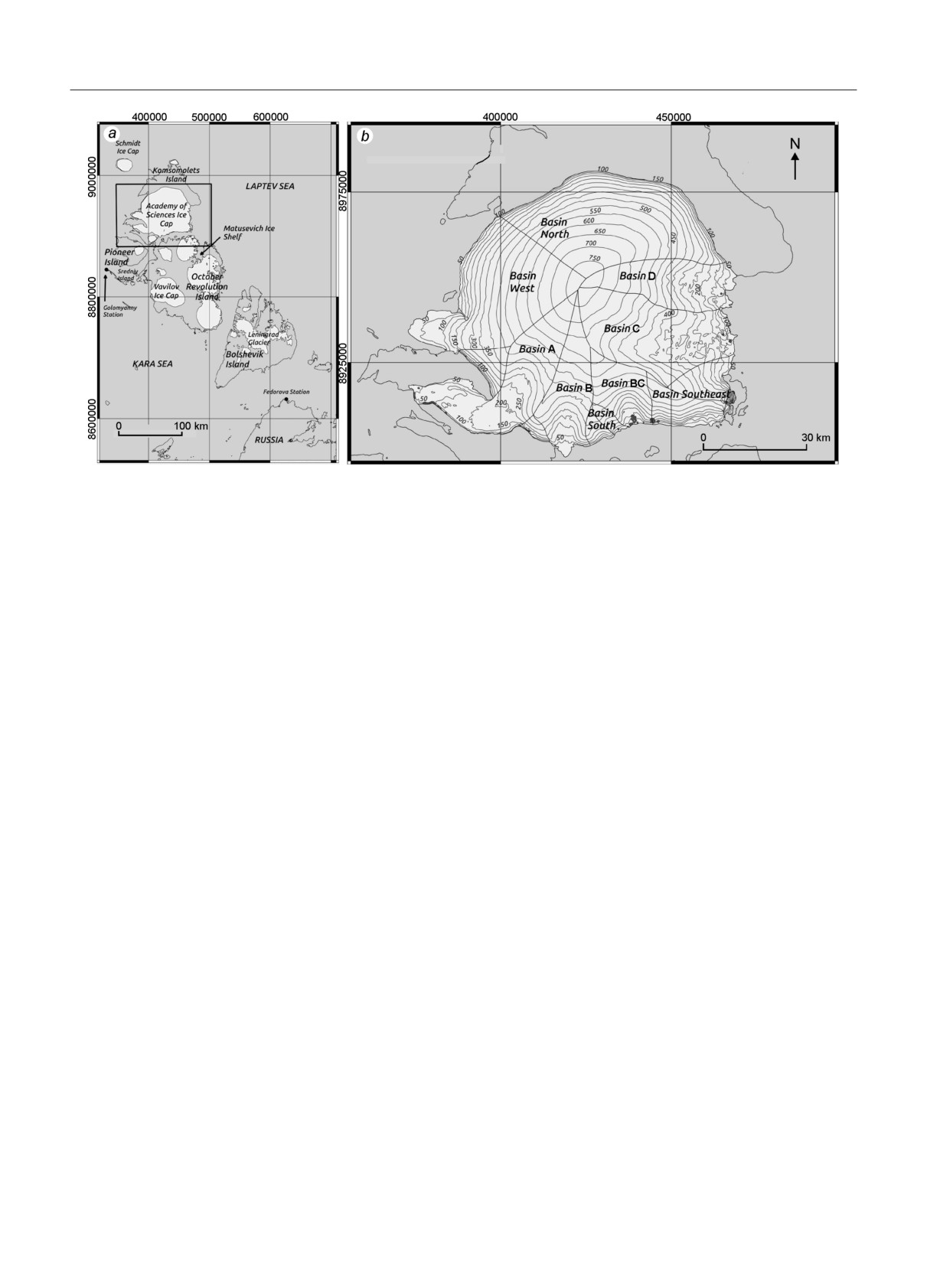
Fig. 1. Location of the Academy of Sciences Ice Cap within Severnaya Zemlya [19] (a), surface topography of the ice

cap (contour level interval is 50 m) and ice divides defining the main basins (b) taken from the Randolph Glacier In

ventory (RGI) version 5.0 [12].

UTM coordinates for zone 47 North are shown

Рис. 1. Местоположение ледникового купола Академии Наук на Северной Земле [19] (а); рельеф поверхности

ледникового купола (горизонтали проведены через 50 м) и ледораздельные линии, ограничивающие основные

ледосборные бассейны (b), показанные в соответствии с Каталогом ледников Рендольф (RGI) версии 5.0 [12].

Дана координатная сетка UTM для северной зоны 47

recent years have attracted more attention to Sever

been pointed out [9, 11]. This, together with the lack

naya Zemlya. First, the collapse of the Matusevich

of studies of intra-annual (including seasonal) varia

Ice Shelf, October Revolution Island (Fig. 1, a), in

tions in the ice-surface velocity of this ice cap, mo

2012, with the subsequent accelerated thinning of the

tivated our work in a previous paper [11]. The latter

glaciers feeding the ice shelf [20]. Second, the «slow»

paper focused on analysing the mentioned short-

surge of the Vavilov Ice Cap, also on October Revo

term variations of ice-surface velocity, and associ

lution Island, in 2015 [21, 22].

ated ice-discharge variations, though also paid atten

There is a limited amount of earlier work on the

tion to other aspects, such as the stress regime, the

dynamics of Severnaya Zemlya glaciers [1, 23, 24],

surface-elevation changes and the long-term varia

and in particular on satellite remote-sensing stud

tions in ice discharge. In the present paper, we ex

ies of glacier surface velocity and ice discharge

pand the discussion by Sánchez-Gámez et al. [11],

from Severnaya Zemlya [1, 9, 25]. More recent

focusing on past and current calving flux estimates of

ly, the increased availability of Synthetic Aperture

the Academy of Sciences Ice Cap and on the possible

Radar (SAR) data, with higher temporal and spa

drivers of the long-term variations of its calving flux.

tial resolution, from platforms such as TerraSAR-X,

PALSAR-1 and Sentinel-1, has allowed further stud

ies [11, 22]. Focusing on the Academy of Sciences

Study site

Ice Cap on Komsomolets Island, Severnaya Zem

lya (see Fig. 1), which is the topic of this paper, the

The Academy of Sciences Ice Cap, located on

available surface velocity and associated calving-

Komsomolets Island, Severnaya Zemlya (see Fig. 1),

flux estimates differ substantially between 1988 and

is one of the largest Arctic ice caps, with an estimated

2009 [1, 9], indicating large interannual to decadal

area of ~5575 km² and volume of ~2184 km³ [1]. Its

variations. However, possible under- and overesti

highest elevation is of ~787 m a.s.l. (ArcticDEM, [26])

mations due to limitations of the available data have

and its maximum ice thickness is of ~819 m [1]. A

 20 

P. Sánchez-Gámez et al.

large fraction (~42%) of the ice-cap margin is marine

SAR acquisitions [34, 35]. For co-registration of the

and ~50% of its bed is below sea level [1].

Sentinel-1 TOPS mode images, we used the Arc

The climate of Severnaya Zemlya is classified as

ticDEM mosaic release 6 [26]. After full co-regis

a polar desert with both low temperatures and low

tration is achieved, deramping of the SLC images

precipitation [9]. The atmospheric circulation is

for correcting the azimuth phase ramp is required

dominated by high-pressure areas over Siberia and

to apply oversampling in the offset-tracking pro

the Arctic Ocean, and low pressure over the Bar

cedures [35]. Once these steps are completed, the

ents and Kara seas [27, 28]. The climatic conditions

offset-tracking technique is the usual one for strip-

are described with more detail in the companion

map mode scenes [34, 36]. We used a matching win

paper [29], as they are more relevant for that study,

dow of 320 × 64 pixels (1200 × 1280 m) in range

focused on mass balance.

and azimuth directions, respectively, with an overs

Regarding the dynamical regime of the ice cap,

ampling factor of two for improving the tracking re

Dowdeswell and Williams [24] found no evidence

sults [34]. The resolution of the final velocity map

of past surge activity within the residence time of

was 130 × 105 m in range and azimuth directions.

the ice, noting that there was no evidence of any de

The geocoding was completed using the ArcticDEM

formation of either large-scale ice structures or me

mosaic product. Errors in surface velocity were esti

dial moraines. Dowdeswell et al. [1] combined ice-

mated by analysing the performance of the algorithm

surface velocities from SAR interferometry of ERS

on ice-free ground on Komsomolets Island under the

tandem-phase scenes from 1995, together with ice-

hypothesis that the error of the offset tracking tech

thickness from radio-echo sounding at 100 MHz, to

nique on bare ground should be close to zero. The

calculate the calving flux from the ice cap. Moho

combined (range and azimuth) root-mean-square

ldt et al. [9], using ICESat altimetry, together with

error in the magnitude of the ice-surface velocity was

older DEMs and velocities from Landsat imagery,

~0,024 m d^-1 (~8,75 m a^-1).

calculated the geodetic mass balance and the calv

Ice thickness data from radio-echo sounding. Ice-

ing flux from the Academy of Sciences Ice Cap for

thickness data were derived from radio-echo sound

various periods during the last three decades. They

ing measurements in spring 1997 using a 100 MHz

showed that the mass balance of the ice cap has been

radar system [1]. The mean crossing-point error in

dominated by variable ice-stream dynamics. Studies

ice-thickness measurements was 10,5 m.

of ice-flow modelling and physical-parameter inver

Dynamic ice discharge and calving flux. We here

sion are also available for the Academy of Sciences

use the term calving flux to denote the ice discharge

Ice Cap [30, 31].

calculated through a flux gate close to the calving

front minus the mass flux involved in front position

changes [37]. In our case study, spanning the peri

Data and Methods

od from November 2016 to November 2017, glacier

terminus position changes have been negligible, so

SAR data and its processing for ice surface veloci-

calving flux and ice discharge are equivalent. We will

ties. We derived the surface velocities on the Acade

most often use the term calving flux, for consistency

my of Sciences Ice Cap from Sentinel-1B SAR TOPS

with previous studies [1, 9].

Interferometric Wide (IW) Level-1 Single Look

For tidewater glaciers, ice discharge is ideally cal

Complex (SLC) images [32]. The resolution when

culated through flux gates as close as possible to the

operating in this mode is 5 of and 20 m in the range

calving fronts, while for floating ice tongues or ice

and azimuth directions, respectively. We used the

shelves it is usually calculated at the grounding line.

vertical transmit and vertical receive (VV) channel,

There is some evidence from both ice-penetrating

which is best suited for retrieval of ice motion [33].

radar data collected in 1997 and earlier investiga

We processed 54 weekly pairs of SAR images, from

tions by Russian scientists that small areas of the ice-

November 2016 to November 2017, with 12-day sep

cap margin at the seaward end of the ice streams of

aration between the images in each pair. Additional

the Academy of Sciences Ice Cap may be floating or

details can be found in [11].

close to floatation [1]. However, we calculated ice

We used the intensity offset-tracking algorithm

discharge at flux gates located within ca. 1,5-3 km of

GAMMA software for processing the Sentinel-1

the calving front, where ice is grounded. Therefore,

 21 

Ледники и ледниковые покровы

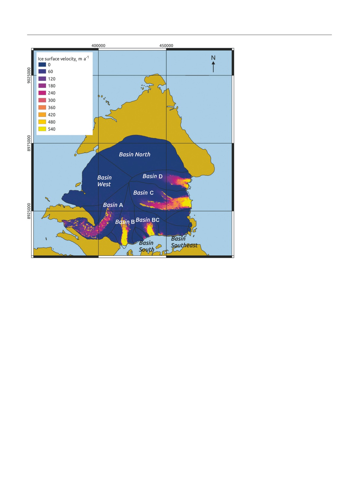
Fig. 2. Surface velocities for the

drainage basins of the Academy of

Sciences Ice Cap, corresponding

to the Sentinel-1 SAR image pair

acquired on 6 and 18 March 2017.

Brown colour indicates ice-free land

areas. The maximum velocities are

1200 m a^-1 for basins B and BC,

1100 m a^-1 for Basin C and 750 m a^-1

for Basin D

Рис. 2. Поверхностные скоро

сти движения в ледосборных

бассейнах ледникового купола

Академии Наук, соответствую

щие паре изображений SAR

Sentinel-1, полученных 6 и

18 марта 2017 г.

Коричневым цветом обозначены

свободные ото льда участки суши.

Максимальные скорости достигают

1200 м/год в бассейнах B и BC,

1100 м/год в бассейне С и 750 м/год

в бассейне D

ice discharge can be calculated as mass flux per unit

was calculated by interpolating the ice-thickness data

time across a given vertical surface S, approximated

of Dowdeswell et al. [1], and was corrected for

using area bins as

surface-elevation changes between 2004 and 2016

from the comparison of ICESat and ArcticDEM

ϕ = ∫

ρv·dS ≈ ∑

ρL_i H_i f v_i cosγ_i,

(1)

strip elevation datasets (see companion paper [20]).

where ρ is the ice density, L_i and H_i are respectively

The velocity vector orientations were calculated with

the width and thickness of an area bin, f is the ratio of

respect to the vector normal to each flux-gate bin.

surface to depth-averaged velocity, v_i is the

Errors in ice discharge were estimated following [7],

magnitude of surface velocity and γ_i is the angle

applying error propagation to Equation 1.

between the surface-velocity vector and the direction

normal to the local flux gate for the bin under

consideration. In general, it is assumed that f ranges

Results

between 0.8 and 1 [38]. Normally, tidewater-glacier

velocity at the terminus is dominated by basal sliding,

Ice cap surface velocity. The surface velocities in

making f close to unity. Following [39], we took

ferred from the Sentinel-1 SAR images are shown in

f = 0.93±0.05, assuming that all tidewater glaciers on

Fig. 2. The marine-terminating drainage basins B,

the Academy of Sciences Ice Cap have a large

BC, C and D show zones of ice-stream-like flow

component of basal motion. For ice density, we

with high velocities, while Basin A also shows a well-

assumed ρ = 900±17 kg m^-3. Our flux gates span the

defined zone of lower, but relatively high velocities.

whole frontal area of each marine-terminating

The surface-velocity fields of all major ice streams,

glacier basin. Each flux gate was divided into small

except A, show a similar pattern. Velocities become

bins of 30 m width. The ice thickness for each bin

prominent where ice flow converges from the upper

 22 

P. Sánchez-Gámez et al.

Table 1. Area, flux gate main characteristics and mean annual (November 2016 - November 2017) calving fluxes for the

marine-terminating drainage basins of the Academy of Sciences Ice Cap shown in Fig. 2. The totals are shown in the last row

Таблица 1. Площади, основные характеристики и среднегодовые (ноябрь 2016 - ноябрь 2017 гг.) расходы льда на айс-

берги ледниковых бассейнов купола Академии Наук, заканчивающихся в море и показанных на рис. 2. В последней

строке даны итоговые значения

Flux gate mean

Flux gate mean surface

Drainage basin

Basin area, km²

Flux gate length, m

Calving flux, Gt a^-1

thickness, m

velocity, m a^-1

West

1033

62 821

174

0,06±0,03

707

7274

251

0,03±0,01

413

5788

441

0,18±0,03

South

14 107

121

0,04±0,02

276

6820

184

384

0,41±0,05

Southeast

359

3740

164

0,08±0,04

829

10 594

223

344

0,69±0,07

475

10 820

171

280

0,44±0,05

Total

4139

155 264

166

1,93±0,12

accumulation areas and increase to a maximum at

while it was clearly evident in the latter. Therefore,

the marine termini. We also calculated the mean an

ice stream flow in Basin BC was initiated after 2002,

nual velocities at the flux gates of all marine-termi

and before 2016.

nating basins, by averaging the 54 pairs of weekly-

The calving flux values shown in Table 1 are an

spaced Sentinel-1 SAR velocities available between

nual averages for the period November 2016 - No

November 2016 and November 2017. These annual-

vember 2017, based on weekly observations along the

averaged velocities, shown in Table 1, were later used

entire year, and thus are not affected by seasonal or

to compute the ice discharge.

other shorter-term intra-annual variations. Sánchez-

Calving flux. The calving flux calculated for each

Gámez et al. [11] have analysed these intra-annual

individual basin of the Academy of Sciences Ice Cap,

variations, which, for certain basins, can reach peak-

for the period November 2016 - November 2017, is

to-peak variations up to ~40% with respect to the

presented in Table 1. The largest contributors are the

mean annual velocity. This indicates that large errors

southern (B and BC) and eastern (C and D) basins,

could be incurred if the ice velocities calculated at a

where the fastest ice streams are located. The total calv

particular snapshot in time were extrapolated to cal

ing flux from the ice cap amounts to 1.93±0.12 Gt a^-1,

culate the calving flux for the whole year.

which is equivalent to -0.35±0.02 m w.e. a^-1 over the

Interannual variability of calving flux. There are

whole area of the ice cap.

available some calving flux estimates for the Acade

my of Sciences Ice Cap, derived using different tech

niques, and corresponding to various periods with

Discussion

in the last ~30 years, some of which partly overlap.

Dowdeswell et al. [1] calculated the calving flux for

Calving flux and its intra-annual variability. Ice

September/December 1995 from SAR interferometry,

Streams A, B, C and D were identified in the earlier

whereas Moholdt et al. [9] did it for the period June

observations by Dowdeswell et al. [1] and Moholdt

2000 - August 2002 using image-matching of Land

et al. [9], but Ice Stream BC, which is currently the

sat scenes. Moholdt et al. [9] also calculated the calv

third largest contributor to total calving flux, was first

ing flux for the periods 1988-2006 and 2003-2009,

noted in our study [11]. Our data thus indicate that

using in these cases an indirect way, subtracting from

fast ice-stream flow was initiated in this basin after

the geodetic mass balance (calculated from DEM dif

the period covered by the two earlier studies and be

ferencing assuming Sorge’s law [40]) an estimate of

fore our study period began in 2017. Sánchez-Gámez

the climatic mass balance. The latter was based on the

et al. [11] additionally compared a Landsat-7 image

assumption that Basin North (basins North and West

of July 2002 with a Sentinel-2 image from March

in our study) is an analogue for the climatic mass bal

2016, and fast flow did not appear in the former,

ance of the entire ice cap [9]. The justification for this

 23 

Ледники и ледниковые покровы

Table 2. Calving fluxes estimated for the drainage basins of the Academy of Sciences Ice Cap for various periods. Basin «North»

here groups our basins North and West, and «Others» groups our basins South, BC and Southeast. These names have been

used for compatibility with [9]

Таблица 2. Расходы льда на айсберги, оценённые за разные периоды для ледосборных бассейнов ледникового купола

Академии Наук. Здесь бассейн «North» включает в себя наши бассейны North и West, а бассейн «Others» - наши бас-

сейны South, BC и Southeast. Эти названия были использованы для возможности сравнения с данными работы [9]

Dowdeswell et al. [1]

Moholdt et al. [9]

This study

Drainage Basin

1995 Gt a^-1

1988-2006 Gt a^-1

2000-2002 Gt a^-1

2003-2009 Gt a^-1

2016/2017 Gt a^-1

Basin North

0,06±0,03

0,03±0,01

0,03

0,5

0,3

0,1

0,18±0,03

0,37

1,9

0,7

0,69±0,07

0,12

0,7

~0,7

0,5

0,44±0,05

Others

~0,1

0,53±0,07

Ice cap total

0,6

3,2

~3,0

1,4

1,93±0,12

assumption is that the northern part of the ice cap is

for the summer warmth at the ice-cap surface [42],

land-terminating, so its climatic and geodetic mass

these large temporal variations in melt-layer content

balances are equal; on the other hand, the western

indicate that the assumption in Sorge’s law of an ab

part of the ice cap, although marine-terminating, is

sence of temporal change in firn thickness or density

dynamically inactive with no significant calving loss

is not suitable for the Academy of Sciences Ice Cap.

es. Extrapolating the estimated climatic mass balance

Further evidence is provided by the modelling exper

to the rest of the ice cap leads to a near-zero climatic

iments on the neighbouring Vavilov Ice Cap on Oc

mass balance for the entire Academy of Sciences Ice

tober Revolution Island, Severnaya Zemlya [43, 44].

Cap. We have made a similar assumption in the com

Even so, the associated uncertainty cannot justify the

panion paper [20], where we discuss other pieces of

large differences in calving flux observed between

evidence supporting this assumption.

the various periods shown in Table 2. For the calving

The available calving flux estimates are shown

flux estimates based on data for particular snapshots

in Table 2. There are significant variations along

in time, the period in the year when the observations

the period analysed, although the calving flux in

were made can neither explain such large differences,

the last decade seems more stable than in previ

considering the magnitude of the seasonal and intra-

ous decades (see Table 2). It is important to remark

annual variability in surface velocities analysed by

that the difference of ~0,5 Gt a^-1 between the esti

Sánchez-Gámez et al. [11]. Hence the need to search

mates for 2003-2009 and 2016-2017 is almost en

for drivers of the large differences in calving flux ob

tirely attributed to the recent initiation of fast flow

served over the last three decades.

in Basin BC [11], which currently accounts for

Drivers of the observed long-term changes in calv-

0.41 ± 0.05 Gt a^-1 (see Table 1). The lowest calving

ing flux. Increasing summer air temperatures may

flux estimate, of 0.6 Gt a^-1 for 1995, could have been

drive an increase of calving flux, through its influ

underestimated, as discussed by Moholdt et al. [9]

ence on surface melting and drainage of meltwater to

and Sánchez-Gámez et al. [11]. The main potential

the glacier bed, enhancing bed lubrication and basal

shortcoming of the indirect estimates of calving flux

sliding [45]. However, such accelerations in veloc

for 1988-2006 and 2003-2009 is the assumption of

ity are mostly short-lived and do not contribute to

Sorge’s law in the conversion from volume changes

increased calving [46]. Air temperatures could still

to mass changes. The analysis by Opel et al. [41] of

play a role if they had an influence on sea-ice or ice

the deep ice core taken in 1999-2001 at the summit

mélange concentration, as these are known to af

of the Academy of Sciences Ice Cap found a strong

fect calving, especially when glaciers are confined

increase in melt-layer content at the beginning of the

in fjords [47, 48]. However, the possible effects of

20th century, which remained at a high level until

sea-ice cover on the dynamics and calving flux of

about 1970 and then decreased markedly until 1998.

the Academy of Sciences Ice Cap are expected to be

As the amount of melt layers in ice cores is a proxy

weak, because their marine termini are not confined

 24 

P. Sánchez-Gámez et al.

in fjords where sea ice or ice mélange could form, be

pography in the terminal zones of the eastern basins

retained and exert a significant backpressure. More

(C and D) [1]. The variations of flux could be associ

over, the seas surrounding Severnaya Zemlya are

ated with changes in floatation conditions [50]. The

characterized by relatively thin first-year ice, as in

floating or near-floating state of these marginal zones

this region new ice is typically produced and soon

has been suggested through various lines of evidence,

moved away by the oceanic currents that flow north

such as the very low ice-surface gradients, the strong

wards past the archipelago [49]. However, Sharov

radar returns from the ice-cap bed in several areas at

and Tyukavina [25] pointed out that medium-term

the margin of the ice streams, and the large numbers

(from decadal to semi-centennial) changes in gla

of tabular icebergs observed near their margins [1].

cier volumes on Severnaya Zemlya were linked to the

extent and duration of sea-ice cover nearby, so that

slow-moving maritime ice caps would grow when the

Conclusions

sea-ice cover in adjacent waters was small, and thin

when the sea-ice cover consolidated. This, however,

The following main conclusions can be drawn

would apply in our case study only to the slow-mov

from our analysis:

ing basins West and A. More generally we did not

1. During the period November 2016 - Novem

find any clear relationship between summer (June-

ber 2017, the marine-terminating margins of the

July-August) average temperature and calving flux,

Academy of Sciences Ice Cap remained nearly sta

or between sea-ice concentration and calving flux,

ble, so that ice discharge and calving flux are equiva

which could explain the observed long-term changes

lent in our study, at 1.93±0.12 Gt a^-1. This is equiva

in calving flux [11]. In fact, the highest calving fluxes

lent to -0.35±0.02 m w.e. a^-1 over the whole area of

corresponded to the period 1988-2006, which had,

the ice cap.

overall, lower air temperatures and larger late Sep

2. The difference of ~0.5 Gt a^-1 between our es

tember sea-ice extent than the periods 2003-2009

timate and that of Moholdt et al. [9] for 2003-2009,

and 2016-2017 [11]. The calving flux in 2003-2009

of ~1.4 Gt a^-1, can be attributed to the initiation,

was lower than that of 2016-2017, and mean summer

sometime between 2002 and 2016, of ice stream flow

temperatures during 2003-2009 (~0,8 °C on average)

in Basin BC, whose current calving flux is estimated

were higher than that of summer 2017 (-0.2 °C). The

to be of 0.41±0.05 Gt a^-1.

mean late September sea-ice extent was also high

3. The long-term (from interannual to inter

er on average for 2003-2009 compared with 2016-

decadal) variations of calving flux during the last three

2017 [11]. Only for the lowest calving flux estimate,

decades have been large, at between 0.6 and 3.2 Gt a^-1.

which corresponds to particular snapshots in time

4. The lack of clear environmental drivers for the

(September and November 1995), did we find that

observed long-term changes of calving flux suggests

the sea-ice extent in late September was larger than

that these variations are an expression of dynamic in

those of the preceding and following years [11]. The

stability, likely associated with intrinsic character

summer before our SAR image acquisitions (2016)

istics of the ice cap. We suggest that this instability

was relatively warm (mean summer air temperature

could be caused by the long-term changes in floata

of 1.2 °C), but was followed by a marked drop in tem

tion conditions associated with the complex geometry

perature, to - 0.2 °C in summer 2017 [11]. However,

of the subglacial and seabed topography in the termi

the sea surrounding northern Severnaya Zemlya was

nal zones of the fast-flowing eastern basins (B and C).

virtually ice free at the end of September 2017 [11].

5. Given that the climatic mass balance has re

In the absence of a clear climate-related driver for

mained close to zero over the last four decades,

the large interannual changes in calving flux observed

in spite of regional warming (see the companion

during the last three decades, we are inclined to asso

paper [20]), the total mass balance of the ice cap has

ciate the observed dynamic instabilities with intrin

been driven mainly by calving flux.

sic characteristics within the Academy of Sciences Ice

Cap, as suggested by Moholdt et al. [9]. One of the

Acknowledgments. This study has received funding

characteristics that could influence long-term varia

from the European Union’s Horizon 2020 research

tions in terminus position and calving fluxes is the

and innovation programme under grant agreement

complex geometry of the subglacial and seabed to

No 727890 and from Agencia Estatal de Investig

 25 

Ледники и ледниковые покровы

ación under grant CTM2017-84441-R of the Spanish

ной сброс льда в море формируют те выводные

Estate Plan for R & D. The radio-echo sounding

ледники, которые дренируют купол в южном и

campaign was funded by grants GR3/9958 and

восточном направлениях. Расхождение с преж

GST/02/2195 to JAD from the UK Natural Environ

ней оценкой расхода льда этого купола в море в

ment Research Council. Copernicus Sentinel data

~1,4 Гт/год, приведённой для 2003-2009 гг. дру

2016-2017 were processed by ESA.

гими авторами, может быть объяснено активиза

цией выводного ледника в ледосборном бассей

не BC, которая произошла где-то между 2002 и

Расширенный реферат

2016 гг. Поскольку изменения положения фрон

тов выводных ледников между обоими периода

Определены поверхностные скорости дви

ми были незначительными, полученные значения

жения ледникового купола Академии Наук на

расходов льда через поперечные сечения в кра

о. Комсомолец (архипелаг Северная Земля в Рос

евых частях эквивалентны айсберговому стоку.

сийской Арктике) в течение периода с ноября

Выполнено сравнение наших результатов оце

2016 г. по ноябрь 2017 г. Для этого использован

нок расхода льда в море с результатами преды

метод оценки смещения элементов с разной ин

дущих исследований и проанализированы воз

тенсивностью отражения на разновременных ра

можные движущие силы тех изменений, которые

дарных изображениях, полученных группировкой

наблюдаются в течение последних трёх десятиле

спутников Sentinel-1. Получены 54 пары недель

тий. Поскольку эти изменения, по-видимому, не

ных скоростей (по двум изображениям в каж

были реакцией на изменения окружающей среды,

дой паре, разделённым 12-дневным периодом).

авторы пришли к выводу, что наблюдаемые из

Общая (по дальности и азимуту) среднеквадра

менения, вероятно, обусловлены внутренними

тичная ошибка в определении скорости движения

характеристиками ледникового купола, которые

поверхности льда составила около 0,024 м/день

регулируют динамику его выводных ледников,

(≈8,75 м/год). Для оценки среднегодового расхода

достигающих моря. В частности, предполагается,

льда в море этого ледникового купола использо

что эта динамическая нестабильность может быть

вано среднее значение этих 54-недельных скоро

вызвана долгосрочными изменениями условий

стей. По нашим оценкам, средний расход льда за

всплывания, связанными со сложной геометри

2016-2017 гг. составил 1,93±0,12 Гт/год, что эк

ей рельефа подледникового ложа и прилегающе

вивалентно потерям -0,35±0,02 м вод. экв. в год

го морского дна в краевых зонах быстротекущих

по всей площади ледникового купола. Основ

выводных ледников с восточной стороны купола.

References

5. McNabb R., Hock R., Huss M. Variations in Alaska

tidewater glacier frontal ablation, 1985-2013. Journ.

1. Dowdeswell J., Bassford R., Gorman M., Williams M.,

of Geophys. Research. 2015, 120 (1): 120-136. doi:

Glazovsky A., Macheret Y., Shepherd A., Vasilenko Y.,

10.1002/2014jf003276.

Savatyuguin L., Hubberten H., Miller H. Form and flow

6. Sánchez-Gámez P., Navarro F.J. Glacier Surface Ve

of the Academy of Sciences Ice Cap, Severnaya Zem

locity Retrieval Using D-InSAR and Offset Tracking

lya, Russian High Arctic. Journ. of Geophys. Research.

Techniques Applied to Ascending and Descending

2002, 107: 1-16. doi: 10.1029/2000jb000129.

Passes of Sentinel-1 Data for Southern Ellesmere Ice

2. Błaszczyk M., Jania J., Hagen J. Tidewater glaciers of

Caps, Canadian Arctic. Remote Sensing. 2017, 9 (5):

Svalbard: recent changes and estimates of calving flux

442. doi: 10.3390/rs9050442.

es. Polish Polar Research. 2009, 30 (2): 85-142.

7. Sánchez-Gámez P., Navarro F.J. Ice discharge error esti

3. Bolch T., Sandberg Sørensen L., Simonsen S.B., Mölg N.,

mates using different cross-sectional area approaches:

Machguth H., Rastner P., Paul F. Mass loss of Green

a case study for the Canadian High Arctic, 2016/17.

land’s glaciers and ice caps 2003-2008 revealed from

Journ. of Glaciology. 2018, 64 (246): 595-608. doi:

ICESat laser altimetry data. Geophys. Research Let

10.1017/jog.2018.48.

ters. 2013, 40: 875-881. doi: 10.1002/grl.50270.

8. De Andrés E., Otero J., Navarro F., Promińska J., La-

4. Burgess E., Forster R., Larsen C. Flow velocities of Alas

pazaran J., Walczowski W. A two-dimensional glacier-

kan glaciers. Nature Communications. 2013, 4: 2146.

fjord coupled model applied to estimate submarine

doi: 10.1038/ncomms3146.

melt rates and front position changes of Hansbreen,

 26 

P. Sánchez-Gámez et al.

Svalbard. Journ. of Glaciology. 2018, 64 (247): 745-

19. Wessel P., Smith W. A global, self-consistent, hier

758, doi: 10.1017/jog.2018.61.

archical, high-resolution shoreline database. Journ.

9. Moholdt G., Heid T., Benham T., Dowdeswell J. Dy

of Geophys. Research. 1996, 101: 8741-8743. doi:

namic instability of marine-terminating glacier ba

10.1029/96JB00104.

sins of Academy of Sciences Ice Cap, Russian High

20. Willis M., Melkonian A., Pritchard M. Outlet glacier

Arctic. Annals of Glaciology. 2012, 53: 193-201. doi:

response to the 2012 collapse of the Matusevich Ice

10.3189/2012aog60a117.

Shelf, Severnaya Zemlya, Russian Arctic. Journ. of

10. Melkonian A., Willis M., Pritchard M., Stewart A. Re

Geophys. Research: Earth Surface. 2015, 120: 2040-

cent changes in glacier velocities and thinning at No

2055. doi: 10.1002/2015jf003544.

vaya Zemlya. Remote Sensing of Environment. 2016,

21. Glazovsky A., Bushueva I., Nosenko G. ‘Slow’ surge of

174: 244-257. doi: 10.1016/j.rse.2015.11.001.

the Vavilov Ice Cap, Severnaya Zemlya. Proc. of the

11. Sánchez-Gámez P., Navarro F., Benham T.,

IASC Workshop on the Dynamics and Mass Balance

Glazovsky A., Bassford R., Dowdeswell J. Intra- and

of Arctic Glaciers, Obergurgl, Austria, 23-25 March

inter-annual variability in dynamic discharge from

2015: 17-18.

the Academy of Sciences Ice Cap, Severnaya Zemlya,

22. Strozzi T., Paul F., Wiesmann A., Schellenberger T.,

Russian Arctic, and its role in modulating mass bal

Kääb A. Circum-Arctic changes in the flow of glaciers

ance. Journ. of Glaciology. 2019, 65 (253): 780-797.

and ice caps from satellite SAR data between the 1990s

doi: 10.1017/jog.2019.58.

and 2017. Remote Sensing. 2017, 9: 947. doi: 10.3390/

12. Pfeffer W., Anthony A., Bliss A., Bolch T., Cogley G.,

rs9090947.

Gardner A., Ove Hagen J., Hock R., Kaser G., Kien-

23. Dowdeswell J., Williams M. Surge-type glaciers in the

holz C., Miles E., Moholdt G., Mölg N., Paul F.,

Russian High Arctic identified from digital satellite

Radić V., Rastner P., Raup B., Rich J., Sharp M.,

imagery. Journ. of Glaciology. 1997, 43: 489-494. doi:

The Randolph Consortium. The Randolph Gla

10.3189/S0022143000035097.

cier Inventory: a globally complete inventory of gla

24. Dowdeswell J., Dowdeswell E., Williams M., Glazov-

ciers. Journ. of Glaciology. 2014, 60: 537-552. doi:

sky A. The glaciology of the Russian High Arctic from

10.3189/2014JoG13J176.

Landsat imagery. U.S. Geological Survey Professional

13. Huss M., Farinotti D. Distributed ice thickness and

Paper. 2010, 1386-F: 94-125.

volume of all glaciers around the globe. Journ. of Geo

25. Sharov A., Tyukavina A. Mapping and interpreting gla

phys. Research: Earth Surface. 2012, 117: 1-10. doi:

cier changes in Severnaya Zemlya with the aid of dif

10.1029/2012jf002523.

ferential interferometry and altimetry. Proc. of Fringe

14. Matsuo K., Heki K. Current ice loss in small glacier

2009 Workshop, Frascati, Italy, 30 November - 4 De

systems of the Arctic islands (Iceland, Svalbard, and

cember 2009, ESA SP-677: 8 p.

the Russian High Arctic) from satellite gravimetry. Ter

26. Noh M.J., Howat I., Porter C., Willis M., Morin P. Arctic

restrial Atmospheric and Oceanic Sciences. 2013, 24:

Digital Elevation Models (DEMs) generated by Surface

657-670. doi: 10.3319/tao.2013.02.22.01(tibxs).

Extraction from TIN-Based Search space Minimization

15. Gardner A., Moholdt G., Cogley J., Wouters B., Ar-

(SETSM) algorithm from RPCs-based Imagery. AGU

endt A., Wahr J., Berthier E., Hock R., Pfeffer W.,

Fall Meeting Abstracts. 2016, EP24C-07.

Kaser G., Ligtenberg S., Bolch T., Sharp M., Ove

27. Alexandrov E., Radionov V., Svyashchennikov P. Snow

Hagen J., van den Broeke M., Paul F. A reconciled es

cover thickness and its measurement in Barents and

timate of glacier contributions to sea level rise: 2003 to

Kara seas. In: Research of climate change and interac

2009. Science. 2013, 340: 852-857. doi: 10.1126/sci

tion processes between ocean and atmosphere in polar

ence.1234532.

regions. Trudy of the Arctic and Antarctic Research In

16. Radić V., Bliss A., Beedlow C., Hock R., Miles E., Co-

stitute. St. Petersburg, 2003, 446: 99-118. [In Russian].

gley G. Regional and global projections of twenty-first

28. Bolshiyanov D., Makeyev V. Arkhipelag Severnaya Zem-

century glacier mass changes in response to climate

lya: Oledeneniye, Istoriya Razvitiya Prirodnoy Sredy.

scenarios from global climate models. Climate Dy

Severnaya Zemlya Archipelago: Glaciation and Histor

namics. 2013, 42: 37-58. doi: 10.1007/s00382-013-

ical Development of the Natural Environment. St. Pe

1719-7.

tersburg: Gidrometeoizdat, 1995: 216 p. [In Russian].

17. Huss M., Hock R. A new model for global glacier

29. Navarro F.J., Sánchez-Gámez P., Glazovsky A.F., Recio-

change and sea-level rise. Frontiers in Earth Science.

Blitz C. Surface-elevation changes and mass balance of

2015, 3: 1-22. doi: 10.3389/feart.2015.00054.

the Academy of Sciences Ice Cap, Severnaya Zemlya.

18. Moholdt G., Wouters B., Gardner A. Recent mass

Led i Sneg. Ice and Snow. 2020, 60 (1): 29-41. doi:

changes of glaciers in the Russian High Arc

10.31857/S2076673420010021

tic. Geophys. Research Letters. 2012, 39: 1-5. doi:

30. Konovalov Y. Inversion for basal friction coefficients

10.1029/2012gl051466.

with a two-dimensional flow line model using Tik

 27 

Ледники и ледниковые покровы

honov regularization. Research in Geophysics. 2012, 2:

40. Bader H. Sorge’s law of densification of snow on high

11. doi: 10.4081/rg.2012.e11.

polar glaciers. Journ. of Glaciology. 1954, 2: 319-323.

31. Konovalov Y., Nagornov O. Two-dimensional prognos

doi: 10.3189/s0022143000025144.

tic experiments for fast-flowing ice streams from the

41. Opel T., Fritzsche D., Meyer H., Schütt R., Weiler K.,

Academy of Sciences Ice Cap. Journ. of Physics. Con

Ruth U., Wilhelms F., Fischer H. 115 year ice-core

ference Series. 2017, 788: 012051. doi: 10.1088/1742-

data from Akademii Nauk Ice Cap, Severnaya Zem

6596/788/1/012051.

lya: high-resolution record of Eurasian Arctic climate

32. Zan F.D., Guarnieri A.M. TOPSAR: Terrain observa

change. Journ. of Glaciology. 2009, 55: 21-31. doi:

tion by progressive scans. IEEE Transactions on Geo

10.3189/002214309788609029.

science and Remote Sensing. 2006, 44 (9): 2352-2360.

42. Koerner R. Devon Island Ice Cap: Core stratigraphy

doi: 10.1109/tgrs.2006.873853.

and paleoclimate. Science. 1977, 196: 15-18. doi:

33. Nagler T., Rott H., Hetzenecker M., Wuite J., Potin P.

10.2307/1744032.

The Sentinel-1 mission: new opportunities for ice sheet

43. Bassford R., Siegert M., Dowdeswell J. Quantify

observations. Remote Sensing. 2015, 7: 9371-9389.

ing the mass balance of Ice Caps on Severnaya Zem

doi: 10.3390/rs70709371.

lya, Russian high Arctic. II: modeling the flow of the

34. Strozzi T., Luckman A., Murray T., Wegmuller U., Wer-

Vavilov Ice Cap under the present climate. Arctic,

ner C. Glacier motion estimation using SAR offset-

Antarctic, and Alpine Research. 2006, 38: 13-20. doi:

tracking procedures. IEEE Transactions on Geosci

10.1657/1523-0430(2006)038[0013:qtmboi]2.0.co;2.

ence and Remote Sensing. 2002, 40: 2384-2391. doi:

44. Bassford R., Siegert M., Dowdeswell J., Oerlemans J.,

10.1109/tgrs.2002.805079.

Glazovsky A., Macheret Y. Quantifying the mass balance

35. Wegmüller U., Werner, C., Strozzi, T., Wiesmann, A.,

of Ice Caps on Severnaya Zemlya, Russian high Arctic.

Othmar, F., Santoro, M. Sentinel-1 support in the

I: climate and mass balance of the Vavilov Ice Cap. Arc

GAMMA software. Proceedings of the FRINGE’15:

tic, Antarctic, and Alpine Research. 2006, 38: 1-12. doi:

Advances in the Science and Applications of SAR In

10.1657/1523-0430(2006)038[0001:qtmboi]2.0.co;2.

terferometry and Sentinel-1 InSAR Workshop, Fra

45. Zwally H.J. Surface melt-induced acceleration of

scati, Italy. 2015: 23-27.

Greenland Ice-Sheet Flow. Science. 2002, 297 (5579):

36. Werner C., Wegmüller U., Strozzi T., Wiesmann A.

218-222. doi: 10.1126/science.1072708.

Precision estimation of local offsets between pairs of

46. Sundal A.V. and 5 others. Melt-induced speed-up

SAR SLCs and detected SAR images. 2005 IEEE In

of Greenland Ice Sheet offset by efficient subglacial

tern. Geoscience and Remote Sensing Symposium

drainage. Nature. 2011, 469 (7331): 521-524. doi:

(IGARSS’05). IEEE Intern. Proceedings. 2005, 7:

10.1038/nature09740.

4803-4805. doi: 10.1109/IGARSS.2005.1526747.

47. Moon T., Joughin I., Smith B. Seasonal to multiyear

37. Cogley, J., Hock R., Rasmussen L., Arendt A., Baud-

variability of glacier surface velocity, terminus posi

er A., Braithwaite R., Jansson P., Kaser G., Möller M.,

tion, and sea ice/ice mélange in northwest Greenland.

Nicholson L., Zemp M. Glossary of glacier mass bal

Journ. of Geophys. Research. Earth. 2015, 120: 818-

ance and related terms. IHP-VII Technical Docu

833. doi: 10.1002/2015jf003494.

ments in Hydrology No. 86, IACS Contribution No. 2,

48. Otero J., Navarro F., Lapazaran J., Welty E., Puczko D.,

UNESCO-IHP, Paris, 2011: 114 p. doi: 10.1017/

Finkelnburg R. Modeling the controls on the front posi

S0032247411000805.

tion of a tidewater glacier in Svalbard. Frontiers in Earth

38. Cuffey K., Paterson S. The Physics of Glaciers, 4th Ed.

Science. 2017, 5:1-11. doi: 10.3389/feart.2017.00029.

Oxford: Butterworth-Heinemann, 2010: 704 p.

49. Serreze M.C., Barry R.G. The Arctic Climate System.

39. Vijay S., Braun M. Seasonal and interannual variability

Cambridge: Cambridge University Press, 2005: 385 p.

of Columbia Glacier, Alaska (2011-2016): Ice velocity,

50. Howat I., Joughin I., Scambos T. Rapid changes in ice

mass flux, surface elevation and front position. Remote

discharge from Greenland outlet glaciers. Science.

Sensing. 2017, 9: 635. doi: 10.3390/rs9060635.

2007, 315: 1559-1561. doi: 10.1126/science.1138478.

 28 